

What is RDBMS and how it is stored in the memory?
How does a relational DBMS internally store its data? In what type of data structure? How does it offer the rapid retrieval without loading the entire database into the main memory (I have heard many DBMS use B-trees)?
A relational database management system (DBMS) typically stores its data in tables, which are made up of rows and columns. Each row represents a single record, and each column represents a field within that record. The data within each column is typically of a specific data type, such as an integer, a string, or a date.Internally, a relational DBMS will use a variety of data structures to store and retrieve this data efficiently. One common data structure used is the B-tree. B-trees are a type of balanced tree data structure that are typically used to store and retrieve large amounts of data in a way that is optimized for disk access.When a query is made to a relational DBMS, the DBMS will use the B-tree to quickly locate and retrieve the requested data without having to load the entire database into main memory. This allows for rapid retrieval of data even when working with very large databases. Additionally, B-trees also help to keep the data in a specific order, which makes it easy and efficient to find a specific piece of data.
How DBMS store the data?
They use B+ trees. B+ tree is a special data structure allowing to efficiently store (i.e. access and update) a large sorted dictionary on a block storage device (i.e. HDD or SSD).
Sorted dictionary is, essentially, a phone book: it allows to locate a random entry by doing a tiny number of steps - i.e. without reading the whole book.
Block storage device can be described very well by a book too:
It's accessed page-by-page (block-by-block)
There is nearly fixed amount of information on each page (block)
You can quickly find a page (block) by its number without need to read anything else. This isn't quite correct for the book - usually you need to see the numbers of few nearby pages to do this. But let's assume we can do this in 1 step.
Reading next or previous page is very fast. This isn't a required property of block storage, but it's good to remember this, since actual block storages we use (HDDs and SSDs) really have it too, and DBMS rely on this fact.
B+ tree is an algorithm (i.e. a set of rules) allowing not just quickly find the entries in phone book, but also:
Add / edit and delete these entries (assuming you can use an eraser)
Maintain desirable page fill ratio - i.e. ensure that % of used space on all pages (except may be 1) in our phone book is higher than desirable limit (usually 75-90%).
As you know, database is a set of tables, and table is a set of indexes. And each index is, essentially, a B+ tree storing its data.
Few examples of how this structure can be mapped to something we know very well:
1. Files and folders:
Database = some root folder
Tables = its subfolders
Indexes = files in each subfolder
2. Bookcase:
Database = bookcase
Table = a book shelf in the bookcase
Index = a book on a shelf
So how table is actually stored as indexes? Let's assume each table has primary key (PK) - a set of columns uniquely identifying any row there. If some table doesn't, we can always add so-called surrogate primary key - a column storing e.g. a very precise time stamp for any particular row showing the moment it was added at.
Since any table has its own primary key (PK), we can store its data as a dictionary sorted by its primary key in B+ tree structure. E.g. if the original table is this one.
Name | Age | State
John | 25 | NY
Jane | 28 | CA
Alex | 33 | CA
Mike | 33 | NY
Its primary index has this structure:
'Alex' -> (33, 'CA')
'Jane' -> (28, 'CA')
'John' -> (25, 'NY')
'Mike' -> (33, 'NY')
As you see, I sorted it in alphabetical order: we store indexes as B+ trees, thus any index is a sorted dictionary as well.
So we know each table has at least primary index, which actually stores the table itself. But there can be other indexes called secondary indexes, that map selected set of columns (secondary index key) to a primary key. Let's see how index on State column (let's call it "IX_State") looks like:
'CA' -> 'Alex'
'CA' -> 'Jane'
'NY' -> 'John'
'NY' -> 'Mike'
It's sorted by State column first, and then by primary key (Name column): normally any index is fully sorted by its key and all columns from the primary key, which aren't part of the secondary key.
How DBMS query the data efficiently?
Let's see how database engine executes this query:
Select Name, State
from People
where State = 'CA'
order by Age
Query translator transforms it to nearly this execution plan:
a = a sequence of all entries from People's table primary index
b = a sequence of entries from a, but where State = 'CA'
c = a sequence of entries from b, but sorted by Aged = a sequence of entries from c, but only Name and State columns
result = d
a, b, c and d are sequences here - i.e. programming abstractions allowing to enumerate all the entries produced by each stage of query execution (an operation of the query execution plan).
Most of operations don't actually store these entries - in fact, they act like Unix pipes sequentially consuming some input and producing the output. Such operations are called streaming operations. Note that index range scan (AKA "index seek") and full index scan (AKA "full scan") are streaming operations, i.e. when a single entry or a sequential range of entries is extracted from index, DBMS doesn't need to even store the result.
But there are some non-streaming operations - they need to read and process the whole result before producing any output. E.g. sorting is non-streaming operation.
To fully clarify these concepts, let's see how above plan could look like, if our database engine would be written in Python:
a = db.get_index('People', 'PK').all()
b = (entry for entry in a if entry['State'] == 'CA')
c = sort(b, 'Age')
d = select(c, 'Name', 'State')
return d
a, b and d are streaming operations here: Index.all() extracts index range (full index), and two others are just Python sequences
c is non-streaming operation, since it requires the whole sequence to be loaded and sorted before it produces the first entry of result.
So it's easy to estimate how much RAM a particular query needs to execute: it's roughly the amount of RAM needed to store all intermediate results of non-streaming operations in query plan. You can assume virtual RAM is used when intermediates don't fit in physical RAM. Actually it's more complex - there are on-disk temporary tables, etc., but it's nearly the same in terms of expected performance.
You may find this is a suboptimal plan: it implies DBMS must read all entries from People's primary index, and also, store full c operation result, since sort is non-streaming operation.
But the good thing is: DBMS passes this initial query plan to a query optimizer, which should transform it to a nearly optimal plan. In our case this plan should be this:
a = entries from People's table IX_State secondary index with 'CA' key
b = a joined with People's table primary index by Name column
c = b sorted by Age
d = select only Name and State columns from c
result = d
Or as Python code:
pk = db.get_index('People', 'PK')
ix_state = db.get_index('People', 'IX_State')a = ix_state.range(point('CA').inclusive(), point('CA').inclusive())
b = (pk.get(entry['Name']) for entry in a)
c = sort(b, 'Age')
d = select(c, 'Name', 'State')
return d
Why this plan is better? Because it processes only a limited number of rows - precisely, all rows with State == 'CA'. Unoptimized query plan processes all rows on steps a and b, so we can predict that optimized plan executes ~ 50x faster (assuming there are 50 states, and people are evenly distributed among them).
Can we improve it? Yes. You might notice that new plan has join operation (step b) - it's necessary, because IX_State doesn't have Age column, but we use it in sort operation. So the only thing DBMS can do here is to join primary index (which always contain all table columns) - as you see in Python's code, "join" here means to do one index lookup per each row in the original data set. Such type of join is called "loop join".
Despite the fact index lookups are fast, joins are relatively costly, since if you join a large data set, you can safely assume DBMS must read approx. one index page in the joined index per each row from the original set. I.e. basically, it will read way more data than it needs: index page usually contains hundreds of entries, but join will discard most of them and use just one from each page, because the chance joined rows come sequentially in the primary index is tiny.
So to improve the efficiency of this query, we can:
1. Add Age column to IX_State index - right after all existing key columns there.
So after adding this column the index should look like this:
('CA', 28) -> 'Jane'
('CA', 33) -> 'Alex'
('NY', 25) -> 'John'
('NY', 33) -> 'Mike'
When it's done, query optimizer won't need to join primary index, since IX_State already has all the data we need, and still can be used to evaluate "where State =='CA'" clause with index seek:
ix_state = db.get_index('People', 'IX_State')
a = ix_state.range(point('CA').inclusive(), point('CA').inclusive())
b = sort(a, 'Age')
c = select(b, 'Name', 'State')
return c
2. We can also remove order by Age clause from the original query - of course, if we don't really need it.
This was a very rough description of how DBMS work. Actually:
There are other types of indexes - e.g. hash and bitmap indexes. But they are used pretty rarely - e.g. InnoDB engine in MySQL supports just B+ trees, and as you know, many of top internet sites (Facebook, Wikipedia, and Quora as well) don't need others to run smoothly. Probably the only other type of index you need to know about is R-tree, which helps to query spatial data (so apps like Google Maps use similar indexes).
I said almost nothing about how query optimizer works, and I'd recommend to read about this too. But again, it's high-level description is simple: it tries to apply different transformations to the query plan to reduce query execution cost (i.e. ~ estimated amount of CPU and IO resources needed to execute the query). There are cases on which query optimizers are bad, so it's good to know about them. E.g. queries with few joins / subqueries are already hard for optimizers, so you can expect suboptimal plans here. Also, there are lots of cases when even optimal plans are hard.
Finally, it's good to know about transactions and transaction isolation. By some reason developers tend to totally ignore this part, but you can save a tremendous amount of time + write way safer code by properly employing these concepts.
DEGREE OF RELATIONS:
Three Types of Relationships in ERD Diagram
There are three types of relationships that can exist between two entities.
An entity-relationship (ER) diagram can be created based on these three types, which are listed below:
one-to-one relationship: In relational database design, a one-to-one (1:1) relationship exists when zero or one instance of entity A can be associated with zero or one instance of entity B, and zero or one instance of entity B can be associated with zero or one instance of entity A. (abbreviated 1:1)
one-to-many relationship: (abbreviated 1:N) In relational database design, a one-to-many (1:N) relationship exists when, for one instance of entity A, there exists zero, one, or many instances of entity B; but for one instance of entity B, there exists zero or one instance of entity A.
many-to-many relationship: In relational database design, a many-to-many (M:N) relationship exists when, for one instance of entity A, there exists zero, one, or many instances of entity B; and for one instance of entity B, there exists zero, one, or many instances of entity A. (abbreviated M:N)
1:n Relationship Explained
A 1:N relationship, often referred to as one-to-many, is a fundamental concept in relational database design. This type of relationship indicates that one record in a given table can be associated with multiple records in another table, yet a record in the second table can only be associated with one record in the first table.
To elaborate, consider two tables, Table A and Table B. In a 1:N relationship, for every single record in Table A, there can be multiple corresponding records in Table B. However, each record in Table B can relate back to only one record in Table A. This is the premise of a one-to-many relationship.
For example, let's imagine Table A is a 'Customers' table, and Table B is an 'Orders' table in a retail database. Each customer (in the Customers table) may place multiple orders (in the Orders table). This establishes a one-to-many relationship from Customers to Orders. However, each order can be linked back to only one customer, maintaining the integrity of the 1:N relationship.
In the realm of table mappings, the 1:N relationship is implemented using a foreign key constraint. A foreign key is a field (or collection of fields) in Table B that uniquely identifies a record in Table A. The foreign key in Table B references the primary key of Table A. This creates a link from the many side (Table B, Orders) to the one side (Table A, Customers), enabling the establishment of the 1:N relationship.
The enforcement of the 1:N relationship in this manner maintains referential integrity in the database, ensuring that relationships between tables remain consistent and the data is reliable. It is crucial to accurately reflect the nature of the relationship between entities during the database design process to ensure the resultant database accurately models the system's requirements.
In summary, a 1:N relationship in the context of table mappings in database design represents a common relational association between two tables, where each record in the first table can relate to multiple records in the second table, and each record in the second table relates back to only one record in the first. This relationship is integral to creating efficient, accurate, and reliable database systems.
Question: Within the context of data modelling, does the notation 1..* have the same meaning as 1:N for the mappings of tables?
In data modeling, different notations are often used to represent the relationships between entities (such as tables in a relational database). The notations "1..*" and "1:N" do, in fact, express the same type of relationship, albeit in different notational systems.
"1..*" Notation: This is commonly used in UML (Unified Modeling Language) diagrams to denote a relationship. The "1.." signifies that one instance of an entity can be associated with zero or more instances of another entity. This notation allows you to specify both minimum and maximum cardinality. In this case, the minimum is one (at least one instance must exist) and the maximum is unspecified (denoted by ''), indicating any number of instances.
Cardinality-\>The number of elements in a set or other grouping, as a property of that grouping.
"1:N" Notation: This notation, commonly used in ER (Entity-Relationship) diagrams, also signifies a relationship between two entities. The "1:N" means that for one instance of an entity, there can be zero, one, or more related instances of another entity. In other words, it denotes a one-to-many relationship.
While the notation differs, both "1..*" and "1:N" represent a one-to-many relationship between two entities. In the context of relational databases, this often translates to a primary key to foreign key relationship between two tables, where one row in the first table can correspond to multiple rows in the second table.
However, one subtle difference lies in the way they handle the lower limit of cardinality. In "1:N", it is usually assumed that the relationship can also be optional on the 'N' side, i.e., there may be instances of the first entity that are not related to any instance of the second entity. But "1.." explicitly states that at least one instance on the '' side must be associated. It's important to interpret and apply these notations within the specific conventions of the modeling methodology you are using.
Following are simple examples of each:
1:1 relationship | In a traditional American marriage, a man can be married to only one woman; a woman can be married to only one man. |
1:N relationship | A child has exactly one biological father; a father can have many biological children. |
M:N relationship | A student can enroll in many classes; a class can have many enrolled students. |
In the business world, one-to-one relationships are few and far between. One-to-many and many-to-many relationships, on the other hand, are common. However, as will be explained later, many-to-many relationships are not permitted in a relational database and must be converted into one-to-many relationships. Relational databases are comprised almost entirely of tables in one-to-many relationships.
Types of Constraints
Limit the number of possible combinations of entities that may participate in a relationship set. There are two types of constraints:
cardinality ratio and
participation constraints.
Very useful concept in describing binary relationship types. For binary relationships, the cardinality ratio must be one of the following types:
1) One To One

An employee can work in at most one department, and a department can have at most one employee.
2) One To Many

An employee can work in many departments (>=0), but a department can have at most one employee.
3) Many To One

An employee can work in at most one department (<=1), and a department can have several employees.
4) Many To Many (default)

An employee can work in many departments (>=0), and a department can have several employees
The following page contains three diagrams describing the 3 relationship types implemented in Microsoft Access.
What is RDBMS (Relational Database Management System)
RDBMS stands for Relational Database Management System.
All modern database management systems like SQL, MS SQL Server, IBM DB2, ORACLE, My-SQL, and Microsoft Access are based on RDBMS.
It is called Relational Database Management System (RDBMS) because it is based on the relational model introduced by E.F. Codd.
How it works
A relational database is the most commonly used database. It contains several tables, and each table has its primary key.
Due to a collection of an organized set of tables, data can be accessed easily in RDBMS.
What is table/Relation?
Everything in a relational database is stored in the form of relations,The RDBMS database uses tables to store data.A table is a collection of related data entries and contains rows and columns to store data.
Each table represents some real-world objects such as person, place, or event about which information is collected. The organized collection of data into a relational table is known as the logical view of the database.
Properties of a Relation:
Each relation has a unique name by which it is identified in the database.
Relation does not contain duplicate tuples.
The tuples of a relation have no specific order.
All attributes in a relation are atomic, i.e., each cell of a relation contains exactly one value.
A table is the simplest example of data stored in RDBMS.
Let's see the example of the student table.
| ID | Name | AGE | COURSE |
| 1 | Ajeet | 24 | B.Tech |
| 2 | aryan | 20 | C.A |
| 3 | Mahesh | 21 | BCA |
| 4 | Ratan | 22 | MCA |
| 5 | Vimal | 26 | BSC |
What is a row or record?
A row of a table is also called a record or tuple. It contains the specific information of each entry in the table. It is a horizontal entity in the table. For example, The above table contains 5 records.
Properties of a row:
No two tuples are identical to each other in all their entries.
All tuples of the relation have the same format and the same number of entries.
The order of the tuple is irrelevant. They are identified by their content, not by their position.
Let's see one record/row in the table.
| ID | Name | AGE | COURSE | | --- | --- | --- | --- | | 1 | Ajeet | 24 | B.Tech |
What is a column/attribute?
A column is a vertical entity in the table which contains all information associated with a specific field in a table. For example, "name" is a column in the above table which contains all information about a student's name.
Properties of an Attribute:
Every attribute of a relation must have a name.
Null values are permitted for the attributes.
Default values can be specified for an attribute automatically inserted if no other value is specified for an attribute.
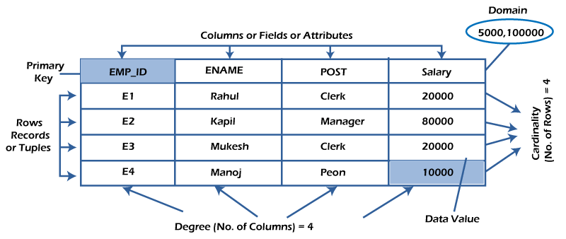
Attributes that uniquely identify each tuple of a relation are the primary key.
| Name | | --- | | Ajeet | | Aryan | | Mahesh | | Ratan | | Vimal |
What is data item/Cells?
The smallest unit of data in the table is the individual data item. It is stored at the intersection of tuples and attributes.
Properties of data items:
Data items are atomic.
The data items for an attribute should be drawn from the same domain.
the below example, the data item in the student table consists of Ajeet, 24 and Btech, etc.
Degree:
The total number of attributes that comprise a relation is known as the degree of the table.
| ID | Name | AGE | COURSE | | --- | --- | --- | --- | | 1 | Ajeet | 24 | B.Tech |
For example, the student table has 4 attributes, and its degree is 4.
| ID | Name | AGE | COURSE |
| 1 | Ajeet | 24 | B.Tech |
| 2 | aryan | 20 | C.A |
| 3 | Mahesh | 21 | BCA |
| 4 | Ratan | 22 | MCA |
| 5 | Vimal | 26 | BSC |
Cardinality:
The total number of tuples at any one time in a relation is known as the table's cardinality. The relation whose cardinality is 0 is called an empty table.
For example, the student table has 5 rows, and its cardinality is 5.
| D | Name | AGE | COURSE |
| 1 | Ajeet | 24 | B.Tech |
| 2 | aryan | 20 | C.A |
| 3 | Mahesh | 21 | BCA |
| 4 | Ratan | 22 | MCA |
| 5 | Vimal | 26 | BSC |
Domain:
The domain refers to the possible values each attribute can contain. It can be specified using standard data types such as integers, floating numbers, etc. For example, An attribute entitled Marital_Status may be limited to married or unmarried values.
NULL Values
The NULL value of the table specifies that the field has been left blank during record creation. It is different from the value filled with zero or a field that contains space.
Data Integrity
There are the following categories of data integrity exist with each RDBMS:
Entity integrity: It specifies that there should be no duplicate rows in a table.
Domain integrity: It enforces valid entries for a given column by restricting the type, the format, or the range of values.
Referential integrity specifies that rows cannot be deleted, which are used by other records.
User-defined integrity: It enforces some specific business rules defined by users. These rules are different from the entity, domain, or referential integrity.
Difference between DBMS and RDBMS
Although DBMS and RDBMS both are used to store information in physical database:
The main differences between DBMS and RDBMS are given below:
| DBMS | RDBMS |
| DBMS applications store data as file. | RDBMS applications store data in a tabular form. |
| In DBMS, data is generally stored in either a hierarchical form or a navigational form. | In RDBMS, the tables have an identifier called primary key and the data values are stored in the form of tables. |
| Normalization is not present in DBMS. | Normalization is present in RDBMS. |
| DBMS does not apply any security with regards to data manipulation. | RDBMS defines the integrity constraint for the purpose of ACID (Atomocity, Consistency, Isolation and Durability) property. |
| DBMS uses file system to store data, so there will be no relation between the tables. | in RDBMS, data values are stored in the form of tables, so a relationship between these data values will be stored in the form of a table as well. |
| DBMS has to provide some uniform methods to access the stored information. | RDBMS system supports a tabular structure of the data and a relationship between them to access the stored information. |
| DBMS does not support distributed database. | RDBMS supports distributed database. |
| DBMS is meant to be for small organization and deal with small data. it supports single user. | RDBMS is designed to handle large amount of data. it supports multiple users. |
| Examples of DBMS are file systems, xml etc. | Example of RDBMS are mysql, postgre, sql server, oracle etc. |
DBMS Architecture
Types of DBMS Architecture
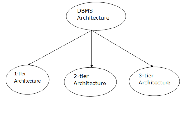
1-Tier Architecture
In this architecture, the database is directly available to the user. It means the user can directly sit on the DBMS and uses it.
Any changes done here will directly be done on the database itself. It doesn't provide a handy tool for end users.
The 1-Tier architecture is used for development of the local application, where programmers can directly communicate with the database for the quick response.
2-Tier Architecture
The 2-Tier architecture is same as basic client-server. In the two-tier architecture, applications on the client end can directly communicate with the database at the server side. For this interaction, API's like: ODBC, JDBC are used.
The user interfaces and application programs are run on the client-side.
The server side is responsible to provide the functionalities like: query processing and transaction management.
To communicate with the DBMS, client-side application establishes a connection with the server side.
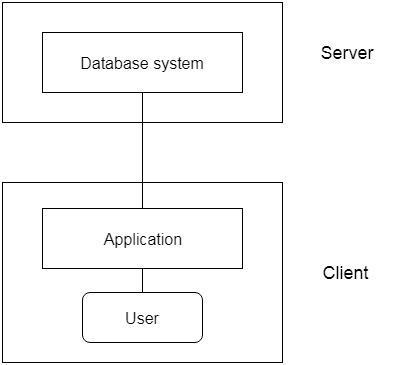
Fig: 2-tier Architecture
3-Tier Architecture
The 3-Tier architecture contains another layer between the client and server. In this architecture, client can't directly communicate with the server.
The application on the client-end interacts with an application server which further communicates with the database system.
End user has no idea about the existence of the database beyond the application server. The database also has no idea about any other user beyond the application.
The 3-Tier architecture is used in case of large web applications.
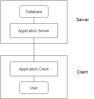
Fig: 3-tier Architecture
Three schema Architecture
The three schema architecture is also called ANSI/SPARC architecture or three-level architecture.
This framework is used to describe the structure of a specific database system.
The three schema architecture is also used to separate the user applications and physical database.
The three schema architecture contains three-levels. It breaks the database down into three different categories.
The three-schema architecture is as follows:
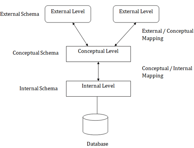
In the above diagram:
It shows the DBMS architecture.
Mapping is used to transform the request and response between various database levels of architecture.
Mapping is not good for small DBMS because it takes more time.
In External / Conceptual mapping, it is necessary to transform the request from external level to conceptual schema.
In Conceptual / Internal mapping, DBMS transform the request from the conceptual to internal level.
Objectives of Three schema Architecture
The main objective of three level architecture is to enable multiple users to access the same data with a personalized view while storing the underlying data only once.
Thus it separates the user's view from the physical structure of the database. This separation is desirable for the following reasons:
Different users need different views of the same data.
The approach in which a particular user needs to see the data may change over time.
The users of the database should not worry about the physical implementation and internal workings of the database such as data compression and encryption techniques, hashing, optimization of the internal structures etc.
All users should be able to access the same data according to their requirements.
DBA should be able to change the conceptual structure of the database without affecting the user's.
Internal structure of the database should be unaffected by changes to physical aspects of the storage.
1. Internal Level
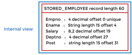
The internal level has an internal schema which describes the physical storage structure of the database.
The internal schema is also known as a physical schema.
It uses the physical data model. It is used to define that how the data will be stored in a block.
The physical level is used to describe complex low-level data structures in detail.
The internal level is generally is concerned with the following activities:
Storage space allocations.
For Example: B-Trees, Hashing etc.Access paths.
For Example: Specification of primary and secondary keys, indexes, pointers and sequencing.Data compression and encryption techniques.
Optimization of internal structures.
Representation of stored fields.
2. Conceptual Level
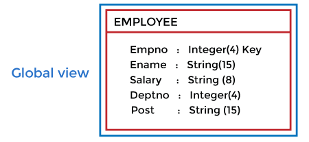
The conceptual schema describes the design of a database at the conceptual level. Conceptual level is also known as logical level.
The conceptual schema describes the structure of the whole database.
The conceptual level describes what data are to be stored in the database and also describes what relationship exists among those data.
In the conceptual level, internal details such as an implementation of the data structure are hidden.
Programmers and database administrators work at this level.
3. External Level

At the external level, a database contains several schemas that sometimes called as subschema. The subschema is used to describe the different view of the database.
An external schema is also known as view schema.
Each view schema describes the database part that a particular user group is interested and hides the remaining database from that user group.
The view schema describes the end user interaction with database systems.
Mapping between Views
The three levels of DBMS architecture don't exist independently of each other. There must be correspondence between the three levels i.e. how they actually correspond with each other. DBMS is responsible for correspondence between the three types of schema. This correspondence is called Mapping.
There are basically two types of mapping in the database architecture:
Conceptual/ Internal Mapping
External / Conceptual Mapping
Conceptual/ Internal Mapping
The Conceptual/ Internal Mapping lies between the conceptual level and the internal level. Its role is to define the correspondence between the records and fields of the conceptual level and files and data structures of the internal level.
External/ Conceptual Mapping
The external/Conceptual Mapping lies between the external level and the Conceptual level. Its role is to define the correspondence between a particular external and the conceptual view.
Data Models
Data Model is the modeling of the data description, data semantics, and consistency constraints of the data. It provides the conceptual tools for describing the design of a database at each level of data abstraction. Therefore, there are following four data models used for understanding the structure of the database:
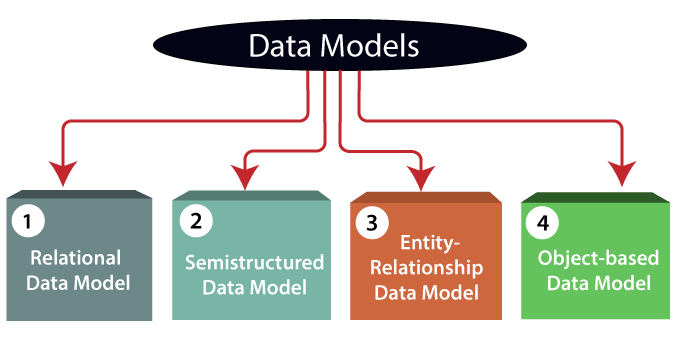
1) Relational Data Model: This type of model designs the data in the form of rows and columns within a table. Thus, a relational model uses tables for representing data and in-between relationships. Tables are also called relations. This model was initially described by Edgar F. Codd, in 1969. The relational data model is the widely used model which is primarily used by commercial data processing applications.
2) Entity-Relationship Data Model: An ER model is the logical representation of data as objects and relationships among them. These objects are known as entities, and relationship is an association among these entities. This model was designed by Peter Chen and published in 1976 papers. It was widely used in database designing. A set of attributes describe the entities. For example, student_name, student_id describes the 'student' entity. A set of the same type of entities is known as an 'Entity set', and the set of the same type of relationships is known as 'relationship set'.
3) Object-based Data Model: An extension of the ER model with notions of functions, encapsulation, and object identity, as well. This model supports a rich type system that includes structured and collection types. Thus, in 1980s, various database systems following the object-oriented approach were developed. Here, the objects are nothing but the data carrying its properties.
4) Semistructured Data Model: This type of data model is different from the other three data models (explained above). The semistructured data model allows the data specifications at places where the individual data items of the same type may have different attributes sets. The Extensible Markup Language, also known as XML, is widely used for representing the semistructured data. Although XML was initially designed for including the markup information to the text document, it gains importance because of its application in the exchange of data.