

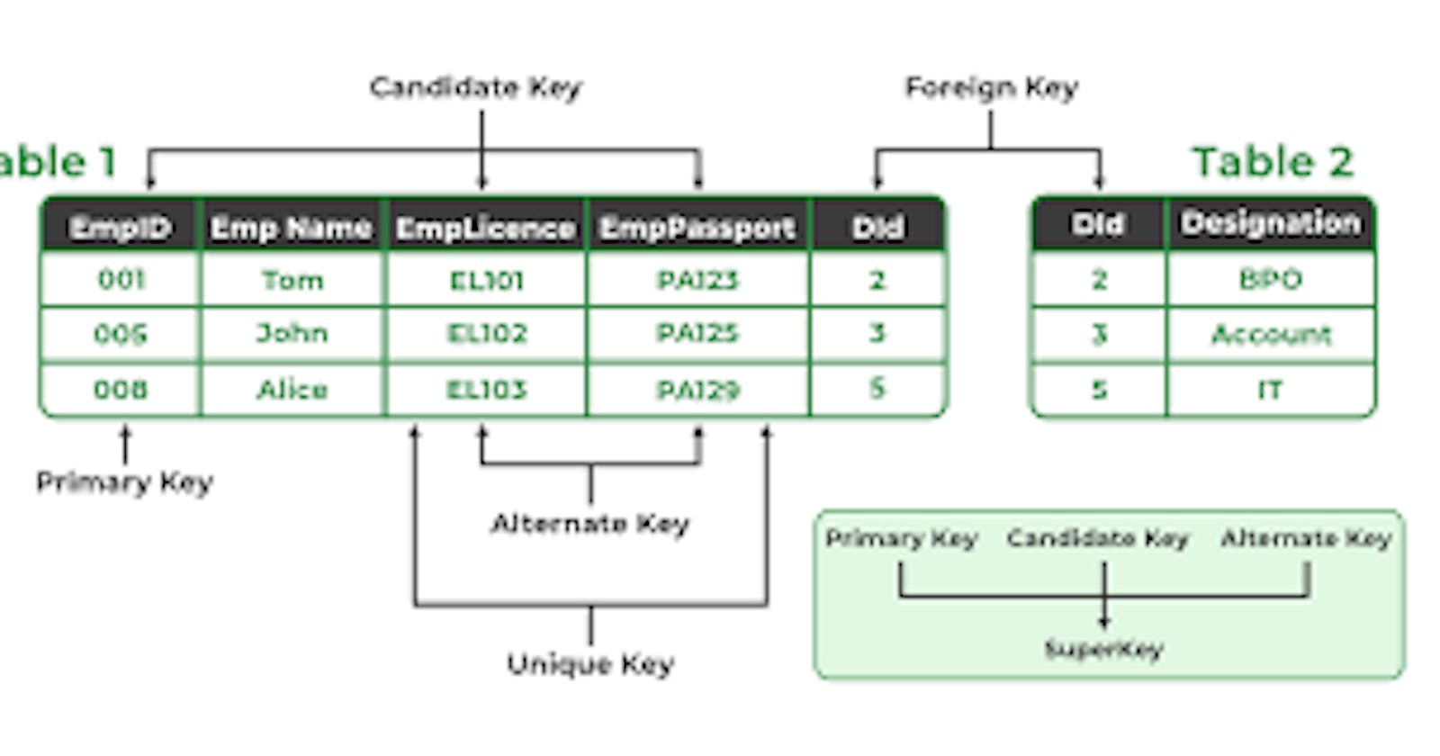
Keys are one of the basic requirements of a relational database model.
used to identify the tuples(rows) uniquely in the table.We also use keys to set up relations amongst various columns and tables of a relational database.
Different Types of Keys in the Relational Model:
-
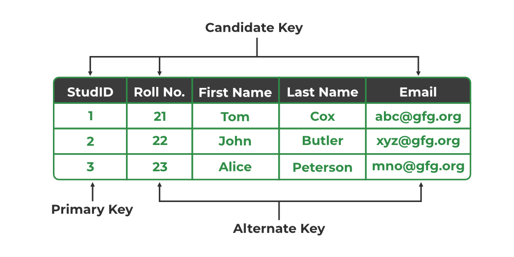
1. Candidate Key: The minimal set of attributes that can uniquely identify a tuple is known as a candidate key. For Example, STUD_NO in STUDENT relation.
It is a minimal super key.
It is a super key with no repeated data is called a candidate key.
The minimal set of attributes that can uniquely identify a record.
It must contain unique values.
It can contain NULL values.
Every table must have at least a single candidate key.
A table can have multiple candidate keys but only one primary key (the primary key cannot have a NULL value, so the candidate key with a NULL value can’t be the primary key).
The value of the Candidate Key is unique and may be null for a tuple.
There can be more than one candidate key in a relationship.
Example:
STUD_NO is the candidate key for relation STUDENT.
Table STUDENT
| STUD_NO | SNAME | ADDRESS | PHONE |
| 1 | Shyam | Delhi | 123456789 |
| 2 | Rakesh | Kolkata | 223365796 |
| 3 | Suraj | Delhi | 175468965 |
- The candidate key can be simple (having only one attribute) or composite as well.
Example:
     {STUD_NO, COURSE_NO} is a composite
     candidate key for relation STUDENT_COURSE.
Table STUDENT_COURSE
| STUD_NO | TEACHER_NO | COURSE_NO |
| 1 | 001 | C001 |
| 2 | 056 | C005 |
Note: In SQL Server a unique constraint that has a nullable column, allows the value ‘null‘ in that column only once. That’s why the STUD_PHONE attribute is a candidate here, but can not be a ‘null’ value in the primary key attribute.
2. Primary Key: There can be more than one candidate key in relation out of which one can be chosen as the primary key. For Example, STUD_NO, as well as STUD_PHONE, are candidate keys for relation STUDENT but STUD_NO can be chosen as the primary key (only one out of many candidate keys).
It is a unique key.
It can identify only one tuple (a record) at a time.
It has no duplicate values, it has unique values.
It cannot be NULL.
Primary keys are not necessarily to be a single column; more than one column can also be a primary key for a table.
Example:
    STUDENT table -> Student(STUD_NO, SNAME,
    ADDRESS, PHONE) , STUD_NO is a primary key
Table STUDENT
| STUD_NO | SNAME | ADDRESS | PHONE |
| 1 | Shyam | Delhi | 123456789 |
| 2 | Rakesh | Kolkata | 223365796 |
| 3 | Suraj | Delhi | 175468965 |
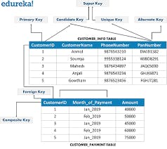
3. Super Key: The set of attributes that can uniquely identify a tuple is known as Super Key. For Example, STUD_NO, (STUD_NO, STUD_NAME), etc. A super key is a group of single or multiple keys that identifies rows in a table. It supports NULL values.
Adding zero or more attributes to the candidate key generates the super key.
A candidate key is a super key but vice versa is not true.
Example:
Consider the table shown above.
STUD_NO+PHONE is a super key.

Relation between Primary Key, Candidate Key, and Super Key
4.Alternate Key: The candidate key other than the primary key is called an alternate key.
All the keys which are not primary keys are called alternate keys.
It is a secondary key.
It contains two or more fields to identify two or more records.
These values are repeated.
Eg:- SNAME, and ADDRESS is Alternate keys
Example:--
Consider the table shown above.
STUD_NO, as well as PHONE both,
are candidate keys for relation STUDENT but
PHONE will be an alternate key
(only one out of many candidate keys).
Primary Key, Candidate Key, and Alternate Key
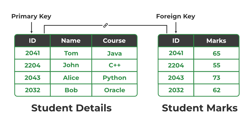
5. Foreign Key: If an attribute can only take the values which are present as values of some other attribute, it will be a foreign key to the attribute to which it refers. The relation which is being referenced is called referenced relation and the corresponding attribute is called referenced attribute the relation which refers to the referenced relation is called referencing relation and the corresponding attribute is called referencing attribute. The referenced attribute of the referenced relation should be the primary key to it.
It is a key it acts as a primary key in one table and it acts as
secondary key in another table.It combines two or more relations (tables) at a time.
They act as a cross-reference between the tables.
For example, DNO is a primary key in the DEPT table and a non-key in EMP
Example:
 Refer Table STUDENT shown above.
 STUD_NO in STUDENT_COURSE is a
 foreign key to STUD_NO in STUDENT relation.
Table STUDENT_COURSE
| STUD_NO | TEACHER_NO | COURSE_NO |
| 1 | 005 | C001 |
| 2 | 056 | C005 |
It may be worth noting that, unlike the Primary Key of any given relation, Foreign Key can be NULL as well as may contain duplicate tuples i.e. it need not follow uniqueness constraint. For Example, STUD_NO in the STUDENT_COURSE relation is not unique. It has been repeated for the first and third tuples. However, the STUD_NO in STUDENT relation is a primary key and it needs to be always unique, and it cannot be null.
Relation between Primary Key and Foreign Key
6.Composite Key: Sometimes, a table might not have a single column/attribute that uniquely identifies all the records of a table. To uniquely identify rows of a table, a combination of two or more columns/attributes can be used. It still can give duplicate values in rare cases. So, we need to find the optimal set of attributes that can uniquely identify rows in a table.
It acts as a primary key if there is no primary key in a table
Two or more attributes are used together to make a composite key.
Different combinations of attributes may give different accuracy in terms of identifying the rows uniquely.
Example:
FULLNAME + DOB can be combined
together to access the details of a student.

Different Types of Keys
FAQs
Why keys are necessary for DBMS?
- Keys are one of the important aspects of DBMS. Keys help us to find the tuples(rows) uniquely in the table. It is also used in developing various relations amongst columns or tables of the database.
What is a Unique Key?
- Unique Keys are the keys that define the record uniquely in the table. It is different from Primary Keys, as Unique Key can contain one NULL value but Primary Key does not contain any NULL values.
What is Artificial Key?
- Artificial Keys are the keys that are used when no attributes contain all the properties of the Primary Key or if the Primary key is very large and complex.
\==========================================================
Database Schema
A database schema is the skeleton structure that represents the logical view of the entire database.It defines how the data is organized and how the relations among them are associated. It formulates all the constraints that are to be applied on the data.
A database schema defines its entities and the relationship among them. It contains a descriptive detail of the database, which can be depicted by means of schema diagrams. It’s the database designers who design the schema to help programmers understand the database and make it useful.
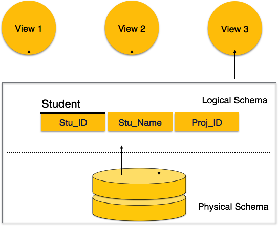
A database schema can be divided broadly into two categories −
Physical Database Schema − This schema pertains to the actual storage of data and its form of storage like files, indices, etc. It defines how the data will be stored in a secondary storage.
Logical Database Schema − This schema defines all the logical constraints that need to be applied on the data stored. It defines tables, views, and integrity constraints.
Database Instance
It is important that we distinguish these two terms individually. Database schema is the skeleton of database. It is designed when the database doesn't exist at all. Once the database is operational, it is very difficult to make any changes to it. A database schema does not contain any data or information.
A database instance is a state of operational database with data at any given time. It contains a snapshot of the database. Database instances tend to change with time. A DBMS ensures that its every instance (state) is in a valid state, by diligently following all the validations, constraints, and conditions that the database designers have imposed.
Mapping from ER Model to Relational Model:-
After designing the ER diagram of system, we need to convert it to Relational models which can directly be implemented by any RDBMS like Oracle, MySQL etc
In this article we will discuss how to convert ER diagram to Relational Model for different scenarios.
Case 1: Binary Relationship with 1:1 cardinality with Total participation of an entity :-

A person has 0 or 1 passport number and Passport is always owned by 1 person. So it is 1:1 cardinality with full participation constraint from Passport.
First Convert each entity and relationship to tables. Person table corresponds to Person Entity with key as Per-Id. Similarly Passport table corresponds to Passport Entity with key as Pass-No. Has Table represents relationship between Person and Passport (Which person has which passport). So it will take attribute Per-Id from Person and Pass-No from Passport.
Person |
| Has |
| Passport | |||
Per-Id | Other Person Attribute | Per-Id | Pass-No | Pass-No | Other PassportAttribute | ||
PR1 | – | PR1 | PS1 | PS1 | – | ||
PR2 | – | PR2 | PS2 | PS2 | – | ||
PR3 | – |
|
|
|
|
|
|
Table 1
As we can see from Table 1, each Per-Id and Pass-No has only one entry in Has Table. So we can merge all three tables into 1 with attributes shown in Table 2. Each Per-Id will be unique and not null. So it will be the key. Pass-No can’t be key because for some person, it can be NULL.
Per-Id | Other Person Attribute | Pass-No | Other PassportAttribute |
Table 2
Case 2: Binary Relationship with 1:1 cardinality and partial participation of both entities

A male marries 0 or 1 female and vice versa as well. So it is 1:1 cardinality with partial participation constraint from both. First Convert each entity and relationship to tables. Male table corresponds to Male Entity with key as M-Id. Similarly Female table corresponds to Female Entity with key as F-Id. Marry Table represents relationship between Male and Female (Which Male marries which female). So it will take attribute M-Id from Male and F-Id from Female.
Male |
| Marry |
| Female | |||
M-Id | Other Male Attribute | M-Id | F-Id | F-Id | Other FemaleAttribute | ||
M1 | – | M1 | F2 | F1 | – | ||
M2 | – | M2 | F1 | F2 | – | ||
M3 | – |
|
|
|
| F3 | – |
Table 3
As we can see from Table 3, some males and some females do not marry. If we merge 3 tables into 1, for some M-Id, F-Id will be NULL. So there is no attribute which is always not NULL. So we can’t merge all three tables into 1. We can convert into 2 tables. In table 4, M-Id who are married will have F-Id associated. For others, it will be NULL. Table 5 will have information of all females. Primary Keys have been underlined.
M-Id | Other Male Attribute | F-Id |
Table 4
F-Id | Other FemaleAttribute |
Table 5
Note: Binary relationship with 1:1 cardinality will have 2 table if partial participation of both entities in the relationship. If atleast 1 entity has total participation, number of tables required will be 1.
Case 3: Binary Relationship with n: 1 cardinality

In this scenario, every student can enroll only in one elective course but for an elective course there can be more than one student. First Convert each entity and relationship to tables. Student table corresponds to Student Entity with key as S-Id. Similarly Elective_Course table corresponds to Elective_Course Entity with key as E-Id. Enrolls Table represents relationship between Student and Elective_Course (Which student enrolls in which course). So it will take attribute S-Id from Student and E-Id from Elective_Course.
Student |
| Enrolls |
| Elective_Course | |||
S-Id | Other Student Attribute | S-Id | E-Id | E-Id | Other Elective CourseAttribute | ||
S1 | – | S1 | E1 | E1 | – | ||
S2 | – | S2 | E2 | E2 | – | ||
S3 | – |
| S3 | E1 |
| E3 | – |
S4 | – |
| S4 | E1 |
|
|
|
Table 6
As we can see from Table 6, S-Id is not repeating in Enrolls Table. So it can be considered as a key of Enrolls table. Both Student and Enrolls Table’s key is same; we can merge it as a single table. The resultant tables are shown in Table 7 and Table 8. Primary Keys have been underlined.
S-Id | Other Student Attribute | E-Id |
Table 7
E-Id | Other Elective CourseAttribute |
Table 8
Case 4: Binary Relationship with m: n cardinality
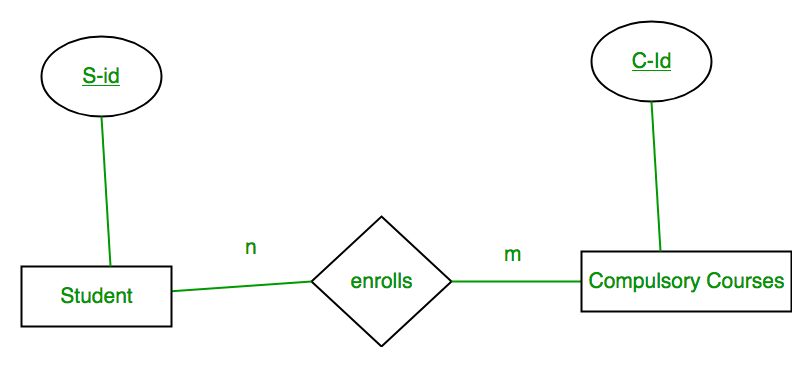
In this scenario, every student can enroll in more than 1 compulsory course and for a compulsory course there can be more than 1 student. First Convert each entity and relationship to tables. Student table corresponds to Student Entity with key as S-Id. Similarly Compulsory_Courses table corresponds to Compulsory Courses Entity with key as C-Id. Enrolls Table represents relationship between Student and Compulsory_Courses (Which student enrolls in which course). So it will take attribute S-Id from Person and C-Id from Compulsory_Courses.
Student |
| Enrolls |
| Compulsory_Courses | |||
S-Id | Other Student Attribute | S-Id | C-Id | C-Id | Other Compulsory CourseAttribute | ||
S1 | – | S1 | C1 | C1 | – | ||
S2 | – | S1 | C2 | C2 | – | ||
S3 | – |
| S3 | C1 |
| C3 | – |
S4 | – |
| S4 | C3 |
| C4 | – |
|
|
| S4 | C2 |
|
|
|
|
|
| S3 | C3 |
|
|
|
Table 9
As we can see from Table 9, S-Id and C-Id both are repeating in Enrolls Table. But its combination is unique; so it can be considered as a key of Enrolls table. All tables’ keys are different, these can’t be merged. Primary Keys of all tables have been underlined.
Case 5: Binary Relationship with weak entity

In this scenario, an employee can have many dependents and one dependent can depend on one employee. A dependent does not have any existence without an employee (e.g; you as a child can be dependent of your father in his company). So it will be a weak entity and its participation will always be total. Weak Entity does not have key of its own. So its key will be combination of key of its identifying entity (E-Id of Employee in this case) and its partial key (D-Name).
First Convert each entity and relationship to tables. Employee table corresponds to Employee Entity with key as E-Id. Similarly Dependents table corresponds to Dependent Entity with key as D-Name and E-Id. Has Table represents relationship between Employee and Dependents (Which employee has which dependents). So it will take attribute E-Id from Employee and D-Name from Dependents.
Employee |
| Has |
| Dependents | ||
E-Id | Other Employee Attribute | E-Id | D-Name | D-Name | E-Id | Other DependentsAttribute |
E1 | – | E1 | RAM | RAM | E1 | – |
E2 | – | E1 | SRINI | SRINI | E1 | – |
E3 | – | E2 | RAM | RAM | E2 | – |
|
| E3 | ASHISH | ASHISH | E3 | – |
Table 10
As we can see from Table 10, E-Id, D-Name is key for Has as well as Dependents Table. So we can merge these two into 1. So the resultant tables are shown in Tables 11 and 12. Primary Keys of all tables have been underlined.
E-Id | Other Employee Attribute |
Table 11
D-Name | E-Id | Other DependentsAttribute |
Table 12
\=======================================================
Relational Operations:-
RELATIONAL ALGEBRA is a widely used procedural query language. It collects instances of relations as input and gives occurrences of relations as output. It uses various operations to perform this action. SQL Relational algebra query operations are performed recursively on a relation. The output of these operations is a new relation, which might be formed from one or more input relations.
Basic SQL Relational Algebra Operations
Relational Algebra divided in various groups
Unary Relational Operations
SELECT (symbol: σ)
PROJECT (symbol: π)
RENAME (symbol: ρ)
Relational Algebra Operations From Set Theory
UNION (υ)
INTERSECTION ( ),
DIFFERENCE (-)
CARTESIAN PRODUCT ( x )
Binary Relational Operations
JOIN
DIVISION
Let’s study them in detail with solutions:
SELECT (σ)
The SELECT operation is used for selecting a subset of the tuples according to a given selection condition. Sigma(σ)Symbol denotes it. It is used as an expression to choose tuples which meet the selection condition. Select operator selects tuples that satisfy a given predicate.
σ<sub>p</sub>(r)
σ is the predicate
r stands for relation which is the name of the table
p is prepositional logic
Example 1
σ topic = "Database" (Tutorials)
Output – Selects tuples from Tutorials where topic = ‘Database’.
Example 2
σ topic = "Database" and author = "DB"( Tutorials)
Output – Selects tuples from Tutorials where the topic is ‘Database’ and ‘author’ is DB.
Example 3
σ sales > 50000 (Customers)
Output– Selects tuples from Customers where sales is greater than 50000
Projection(π)
The projection eliminates all attributes of the input relation but those mentioned in the projection list. The projection method defines a relation that contains a vertical subset of Relation.
This helps to extract the values of specified attributes to eliminates duplicate values. (pi) symbol is used to choose attributes from a relation. This operator helps you to keep specific columns from a relation and discards the other columns.
Example of Projection:
Consider the following table
| CustomerID | CustomerName | Status |
| 1 | Active | |
| 2 | Amazon | Active |
| 3 | Apple | Inactive |
| 4 | Alibaba | Active |
Here, the projection of CustomerName and status will give
Π CustomerName, Status (Customers)
| CustomerName | Status |
| Active | |
| Amazon | Active |
| Apple | Inactive |
| Alibaba | Active |
Rename (ρ)
Rename is a unary operation used for renaming attributes of a relation.
ρ (a/b)R will rename the attribute ‘b’ of relation by ‘a’.
Union operation (υ)
UNION is symbolized by ∪ symbol. It includes all tuples that are in tables A or in B. It also eliminates duplicate tuples. So, set A UNION set B would be expressed as:
The result <- A ∪ B
For a union operation to be valid, the following conditions must hold –
R and S must be the same number of attributes.
Attribute domains need to be compatible.
Duplicate tuples should be automatically removed.
Example
Consider the following tables.
Table A | Table B | |||
|---|---|---|---|---|
column 1 | column 2 | column 1 | column 2 | |
1 | 1 | 1 | 1 | |
1 | 2 | 1 | 3 |
A ∪ B gives
| Table A ∪ B | |
| column 1 | column 2 |
| 1 | 1 |
| 1 | 2 |
| 1 | 3 |
Set Difference (-)
– Symbol denotes it. The result of A – B, is a relation which includes all tuples that are in A but not in B.
The attribute name of A has to match with the attribute name in B.
The two-operand relations A and B should be either compatible or Union compatible.
It should be defined relation consisting of the tuples that are in relation A, but not in B.
Example
A-B
| Table A – B | |
| column 1 | column 2 |
| 1 | 2 |
Intersection
An intersection is defined by the symbol ∩
A ∩ B
Defines a relation consisting of a set of all tuple that are in both A and B. However, A and B must be union-compatible.
 Visual Definition of Intersection
Example:
A ∩ B
| Table A ∩ B | |
| column 1 | column 2 |
| 1 | 1 |
Cartesian Product(X) in DBMS
Cartesian Product in DBMS is an operation used to merge columns from two relations. Generally, a cartesian product is never a meaningful operation when it performs alone. However, it becomes meaningful when it is followed by other operations. It is also called Cross Product or Cross Join.
Example – Cartesian product
σ column 2 = ‘1’ (A X B)
Output – The above ex
ample shows all rows from relation A and B whose column 2 has value 1
| σ column 2 = ‘1’ (A X B) | | --- | | column 1 | column 2 | | 1 | 1 | | 1 | 1 |
Join Operations
Join operation is essentially a cartesian product followed by a selection criterion.
Join operation denoted by ⋈.
JOIN operation also allows joining variously related tuples from different relations.
Types of JOIN:
Various forms of join operation are:
Inner Joins:
Theta join
EQUI join
Natural join
Outer join:
Left Outer Join
Right Outer Join
Full Outer Join
Inner Join:
In an inner join, only those tuples that satisfy the matching criteria are included, while the rest are excluded. Let’s study various types of Inner Joins:
1)Theta Join:
The general case of JOIN operation is called a Theta join. It is denoted by symbol θ
Example
A ⋈θ B
Theta join can use any conditions in the selection criteria.
For example:
A ⋈ A.column 2 > B.column 2 (B)
| A ⋈ A.column 2 > B.column 2 (B) | |
| column 1 | column 2 |
| 1 | 2 |
2)EQUI join:
When a theta join uses only equivalence condition, it becomes a equi join.
For example:
A ⋈ A.column 2 = B.column 2 (B)
| A ⋈ A.column 2 = B.column 2 (B) | |
| column 1 | column 2 |
| 1 | 1 |
EQUI join is the most difficult operations to implement efficiently using SQL in an RDBMS and one reason why RDBMS have essential performance problems.
3)NATURAL JOIN (⋈)
Natural join can only be performed if there is a common attribute (column) between the relations. The name and type of the attribute must be same.
Example
Consider the following two tables
| C | |
| Num | Square |
| 2 | 4 |
| 3 | 9 |
| D | |
| Num | Cube |
| 2 | 8 |
| 3 | 27 |
C ⋈ D
| C ⋈ D | ||
| Num | Square | Cube |
| 2 | 4 | 8 |
| 3 | 9 | 27 |
OUTER JOIN
In an outer join, along with tuples(rows) that satisfy the matching criteria, we also include some or all tuples that do not match the criteria.
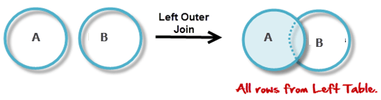
Left Outer Join(A B)
In the left outer join, operation allows keeping all tuple in the left relation. However, if there is no matching tuple is found in right relation, then the attributes of right relation in the join result are filled with null values.
Consider the following 2 Tables
| A | |
| Num | Square |
| 2 | 4 |
| 3 | 9 |
| 4 | 16 |
| B | |
| Num | Cube |
| 2 | 8 |
| 3 | 18 |
| 5 | 75 |
A B
| A ⋈ B | ||
| Num | Square | Cube |
| 2 | 4 | 8 |
| 3 | 9 | 18 |
| 4 | 16 | – |
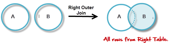
Right Outer Join: ( A B )
In the right outer join, operation allows keeping all tuple in the right relation. However, if there is no matching tuple is found in the left relation, then the attributes of the left relation in the join result are filled with null values.
A B
| A ⋈ B | ||
| Num | Cube | Square |
| 2 | 8 | 4 |
| 3 | 18 | 9 |
| 5 | 75 | – |
Full Outer Join: ( A B)
In a full outer join, all tuples from both relations are included in the result, irrespective of the matching condition.
A B
| A ⋈ B | ||
| Num | Cube | Square |
| 2 | 4 | 8 |
| 3 | 9 | 18 |
| 4 | 16 | – |
| 5 | – | 75 |
Summary
| Operation(Symbols) | Purpose |
| Select(σ) | The SELECT operation is used for selecting a subset of the tuples according to a given selection condition |
| Projection(π) | The projection eliminates all attributes of the input relation but those mentioned in the projection list. |
| Union Operation(∪) | UNION is symbolized by symbol. It includes all tuples that are in tables A or in B. |
| Set Difference(-) | – Symbol denotes it. The result of A – B, is a relation which includes all tuples that are in A but not in B. |
| Intersection(∩) | Intersection defines a relation consisting of a set of all tuple that are in both A and B. |
| Cartesian Product(X) | Cartesian operation is helpful to merge columns from two relations. |
| Inner Join | Inner join, includes only those tuples that satisfy the matching criteria. |
| Theta Join(θ) | The general case of JOIN operation is called a Theta join. It is denoted by symbol θ. |
| EQUI Join | When a theta join uses only equivalence condition, it becomes a equi join. |
| Natural Join(⋈) | Natural join can only be performed if there is a common attribute (column) between the relations. |
| Outer Join | In an outer join, along with tuples that satisfy the matching criteria. |
| Left Outer Join( ) | In the left outer join, operation allows keeping all tuple in the left relation. |
| Right Outer join() | In the right outer join, operation allows keeping all tuple in the right relation. |
| Full Outer Join() | In a full outer join, all tuples from both relations are included in the result irrespective of the matching condition. |